Overview
In this assignment, I analyzed a large NOAA climate dataset containing over 17 million temperature measurements from weather stations around the world. Using R and the tidyverse, I cleaned the data, filtered by country and time period, and visualized global temperature trends over time.
Key tasks:
- Imported and cleaned NOAA temperature data (17.9M rows)
- Filtered data for Japan and Algeria (2000–2025)
- Summarized temperature statistics by year and country
- Visualized mean, min, and max temperature trends over time
Problem 1: Import the data
First, I loaded the three required CSV files into RStudio. I saved them as temperatures, stations, and countries.
Rows: 17,911,764
Columns: 4
$ ID      <chr> "ACW00011604", "ACW00011604", "ACW00011604", "ACW00011604", "A…
$ Year    <dbl> 1961, 1961, 1961, 1961, 1961, 1961, 1961, 1961, 1961, 1961, 19…
$ Month   <dbl> 1, 2, 3, 4, 5, 6, 7, 8, 9, 10, 11, 12, 1, 2, 3, 4, 5, 6, 7, 8,…
$ AvgTemp <dbl> -142, 183, 419, 720, 1075, 1546, 1517, 1428, 1360, 1121, 457, …
Rows: 27,585
Columns: 5
$ ID        <chr> "ACW00011604", "AE000041196", "AEM00041184", "AEM00041194", …
$ LATITUDE  <dbl> 57.7667, 25.3330, 25.6170, 25.2550, 24.4300, 24.4330, 24.262…
$ LONGITUDE <dbl> 11.8667, 55.5170, 55.9330, 55.3640, 54.4700, 54.6510, 55.609…
$ STNELEV   <dbl> 18.0, 34.0, 31.0, 10.4, 3.0, 26.8, 264.9, 3366.0, 378.0, 977…
$ NAME      <chr> "SAVE", "SHARJAH_INTER_AIRP", "RAS_AL_KHAIMAH_INTE", "DUBAI_…
Rows: 279
Columns: 2
$ `FIPS 10-4` <chr> "AF", "AX", "AL", "AG", "AQ", "AN", "AO", "AV", "AY", "AC"…
$ Name        <chr> "Afghanistan", "Akrotiri", "Albania", "Algeria", "American…
Problem 2: Clean the data
For problem 2, I cleaned the data as required. In the temperature file, I removed those rows that are -9999. AvgTemp is stored as “hundredths of a degree”, so I divided by 100 to get real °C. Also, I created a country code column from the first two letters of the station ID. Then I removed duplicate country codes so each code only shows once.
# A tibble: 0 × 2
# ℹ 2 variables: FIPS 10-4 <chr>, n <int>
Problem 3: Set parameters
For problem 3, I set my own parameters country, year begin, year end and month. This makes it easy to change the query without rewriting the whole code.
# A tibble: 1 × 5
  data_file     country year_begin year_end month
  <chr>         <chr>        <dbl>    <dbl> <dbl>
1 my_output.csv Japan         2000     2025     1
Problem 4: Join + Filter (Japan)
For Problem 4, I joined the datasets and then filtered the data using my parameters. I selected the required columns, sorted by station NAME, and showed the first 7 and last 7 rows. Finally, I saved the result as a CSV file.
# A tibble: 7 × 7
  NAME     LATITUDE LONGITUDE Country  Year Month AvgTemp
  <chr>       <dbl>     <dbl> <chr>   <dbl> <dbl>   <dbl>
1 ABASHIRI     44.0      144. Japan    2000     1   -4.8
2 ABASHIRI     44.0      144. Japan    2001     1   -7.57
3 ABASHIRI     44.0      144. Japan    2002     1   -4.4
4 ABASHIRI     44.0      144. Japan    2003     1   -6.1
5 ABASHIRI     44.0      144. Japan    2004     1   -4.1
6 ABASHIRI     44.0      144. Japan    2005     1   -5.68
7 ABASHIRI     44.0      144. Japan    2006     1   -6
# A tibble: 7 × 7
  NAME  LATITUDE LONGITUDE Country  Year Month AvgTemp
  <chr>    <dbl>     <dbl> <chr>   <dbl> <dbl>   <dbl>
1 YORON     27.0      128. Japan    2019     1    17.8
2 YORON     27.0      128. Japan    2020     1    18.2
3 YORON     27.0      128. Japan    2021     1    16.6
4 YORON     27.0      128. Japan    2022     1    17.3
5 YORON     27.0      128. Japan    2023     1    17.2
6 YORON     27.0      128. Japan    2024     1    17.7
7 YORON     27.0      128. Japan    2025     1    16.3
Problem 4 (Repeat): Join + Filter (Algeria)
Then I repeated the same steps for Algeria (2000–2025, June) and saved it to a different CSV file.
# A tibble: 7 × 7
  NAME  LATITUDE LONGITUDE Country  Year Month AvgTemp
  <chr>    <dbl>     <dbl> <chr>   <dbl> <dbl>   <dbl>
1 ADRAR     27.9     -0.28 Algeria  2000     6    34.3
2 ADRAR     27.9     -0.28 Algeria  2001     6    35.6
3 ADRAR     27.9     -0.28 Algeria  2003     6    35.3
4 ADRAR     27.9     -0.28 Algeria  2004     6    33.8
5 ADRAR     27.9     -0.28 Algeria  2005     6    34.4
6 ADRAR     27.9     -0.28 Algeria  2006     6    35.1
7 ADRAR     27.9     -0.28 Algeria  2007     6    34.1
# A tibble: 7 × 7
  NAME   LATITUDE LONGITUDE Country  Year Month AvgTemp
  <chr>     <dbl>     <dbl> <chr>   <dbl> <dbl>   <dbl>
1 ZENATA     35.0     -1.45 Algeria  2019     6    22.1
2 ZENATA     35.0     -1.45 Algeria  2020     6    23.2
3 ZENATA     35.0     -1.45 Algeria  2021     6    23.0
4 ZENATA     35.0     -1.45 Algeria  2022     6    24.6
5 ZENATA     35.0     -1.45 Algeria  2023     6    24.4
6 ZENATA     35.0     -1.45 Algeria  2024     6    22.9
7 ZENATA     35.0     -1.45 Algeria  2025     6    26.7
Problem 5: Summaries
For Problem 5, I summarized the joined data. I made three tables: summary_year, coverage_year, and coverage_country. Then I reported the number of measurements in 2025 and the top 5 countries overall.
# A tibble: 1 × 2
   Year n_measurements
  <dbl>          <int>
1  2025         126155
# A tibble: 5 × 2
  Name          n_measurements
  <chr>                  <int>
1 United States        7810379
2 Canada               1540423
3 Russia                788220
4 Australia             760851
5 Germany               518642
# A tibble: 1 × 2
  min_year max_year
     <dbl>    <dbl>
1     1701     2026
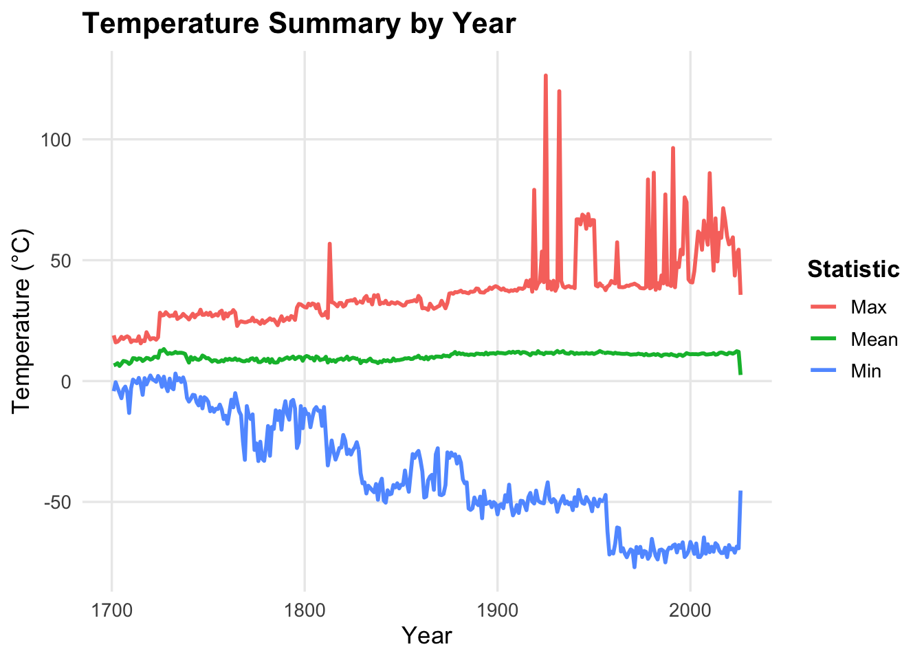
Problem 6: Plot
For Problem 6, I made a line plot using the yearly summary table. It shows the mean, min, and max temperature over time.